《物理化学实验》-生态环境系

misaraty 收录于学术

2023-09-19 约 2619 字预计阅读 6 分钟

前言

此课程由化学与材料科学学院负责，面向生态环境系环工、环科本科生。
教学地点：化学楼402实验室
主要教材：《基础化学实验4——物性参数与测定》马志广、庞秀言主编化学工业出版社 2016年
百度网盘下载或Github下载，包含教案、数据绘图文件、电导率仪说明书、学生实验报告示例等。

电导法测定弱电解质的电离平衡常数

实验思路

本实验需要测量乙酸的电离平衡常数，而电离平衡常数与浓度有关（见P65，式（1））。因涉及到弱电解质乙酸，所以浓度需要考虑电离度α。
采用电导法测定电离度α（见P66，式（6））。
依据式（7）画图，先求得截距，再根据斜率求出电离平衡常数。

数据处理

学习三线表的标准格式，实验报告、论文等表格应遵循三线表格式要求。
表格易错处

警告

表2 电导率测定结果

κ（HAc）=κ（溶液）-κ（水）
κ（水）一般小于10 µS·cm-1，即10*10-4 S·m-1
求解1/Λm(HAc)时，考虑Λm=κ/c。
求解cΛm(HAc)/c⊖时，考虑c⊖=1000 mol/m3。

Origin作图

λm-1为y，cλm/c⊖为x，填写Book1。

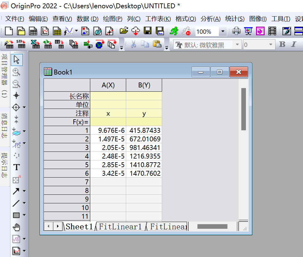
选中作图所需的数据，点击绘图-散点图。

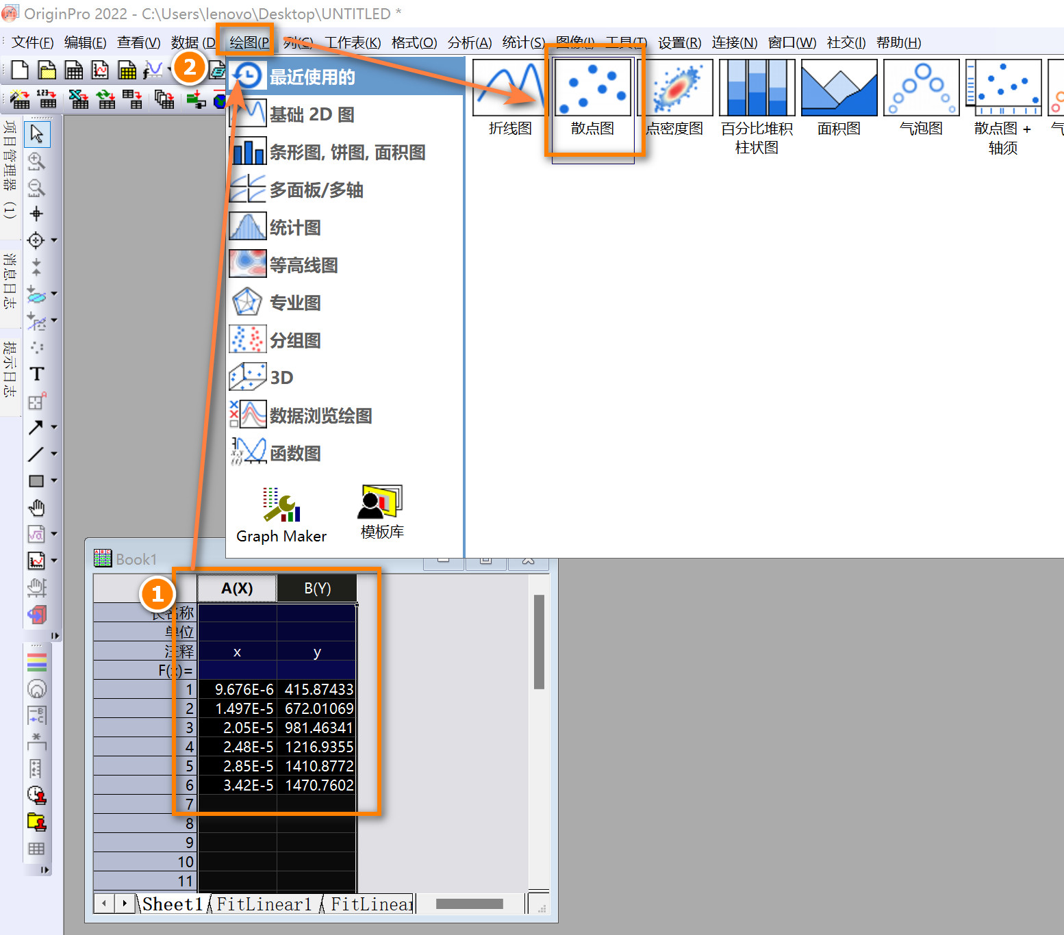
选中分析-拟合-线性拟合，获得线性拟合方程。

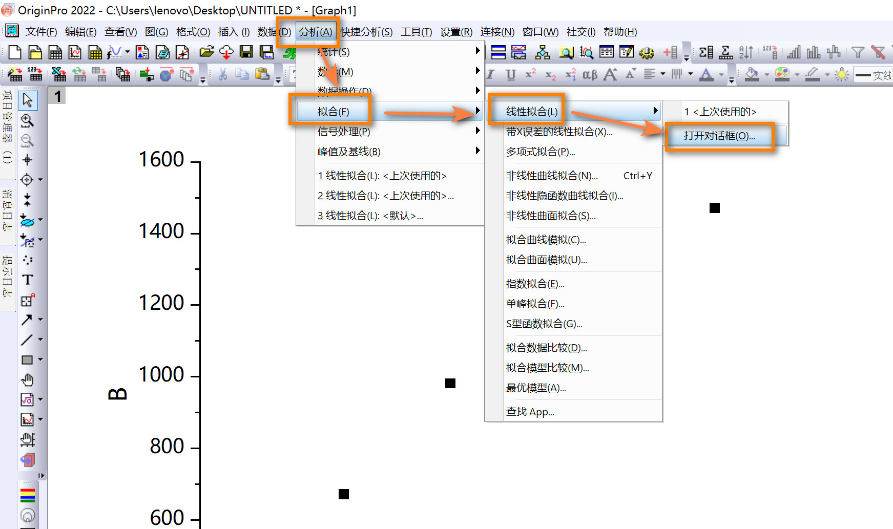
双击图中对应的位置，修改图的坐标轴等。

警告

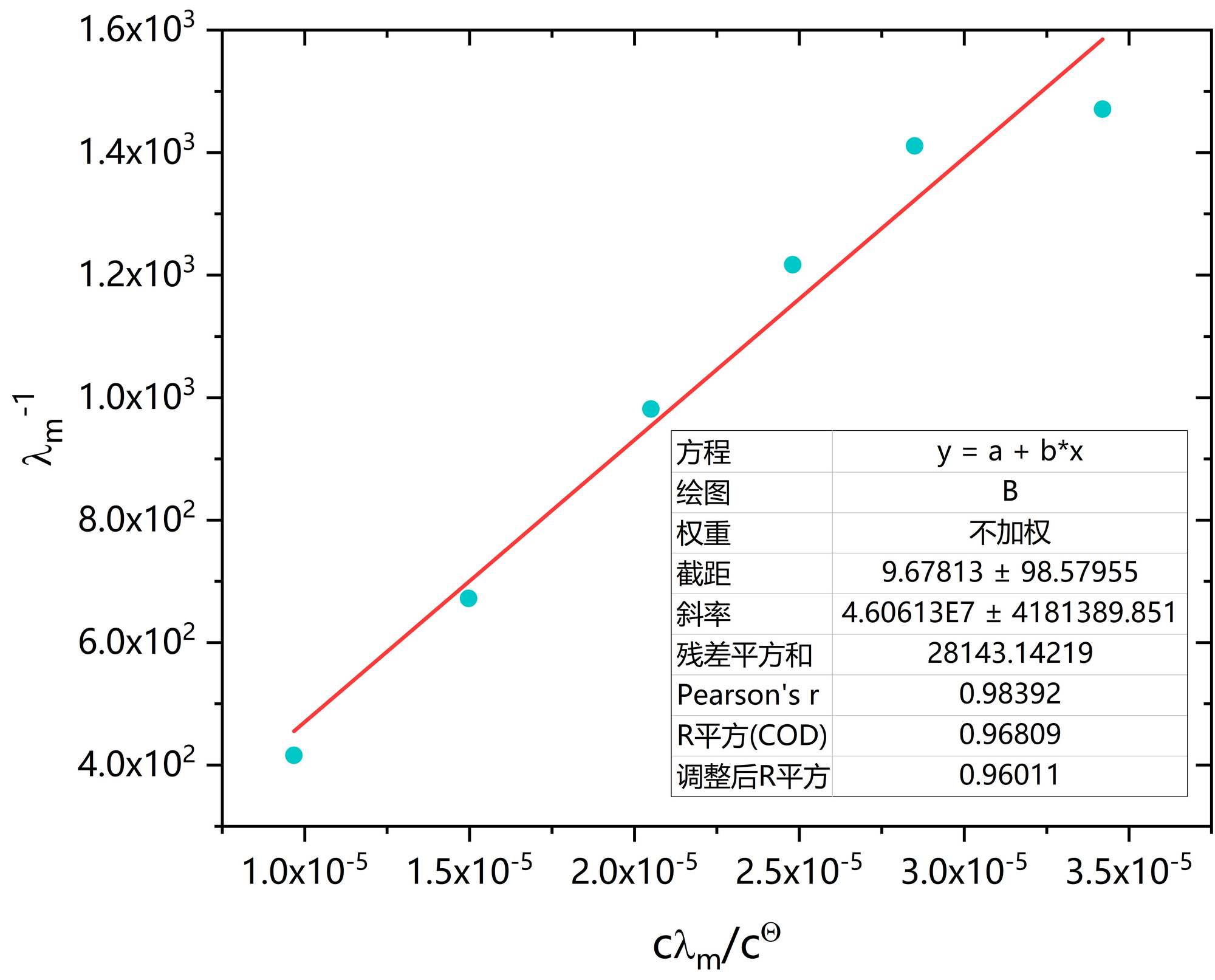
Origin出图显示demo是因为破解不完全所致。
x轴、y轴单位别遗漏，此实验的图都有这个bug。

Python作图

代码：

 1
 2
 3
 4
 5
 6
 7
 8
 9
10
11
12
13
14
15
16
17
18
19
20
21
22
23
24
25
26
27
28
29
30
31
32
33
34
35
36


#!/usr/bin/env python
# -*-coding:utf-8 -*-

import os
import numpy as np
import matplotlib.pyplot as plt
os.chdir(os.path.split(os.path.realpath(__file__))[0])

# 数据
data = [
    [9.676E-6, 415.87433],
    [1.497E-5, 672.01069],
    [2.05E-5, 981.46341],
    [2.48E-5, 1216.93548],
    [2.85E-5, 1410.87719],
    [3.42E-5, 1470.76023]
]

x, y = zip(*data)

# 拟合数据
coefs = np.polyfit(x, y, 1)
fit_func = np.poly1d(coefs)

# 绘图
plt.scatter(x, y, color='tab:blue', label='Data Points')
plt.plot(x, fit_func(x), color='tab:red', label=f'Fit: y = {coefs[0]:.4f}x + {coefs[1]:.4f}')
plt.xlabel(r'$c \times \frac{\Lambda_m}{c^{\ominus}}$')
plt.ylabel(r'$\frac{1}{\Lambda_m}$')
plt.legend()
plt.grid(True)

# 保存到本地
plt.tight_layout()
plt.savefig("result.jpg", dpi=300)
plt.show()

作图：

Matlab作图

代码：

 1
 2
 3
 4
 5
 6
 7
 8
 9
10
11
12
13
14
15
16
17
18
19
20
21
22
23
24
25
26
27
28
29
30
31


% 数据
data = [
    9.676E-6, 415.87433;
    1.497E-5, 672.01069;
    2.05E-5, 981.46341;
    2.48E-5, 1216.93548;
    2.85E-5, 1410.87719;
    3.42E-5, 1470.76023
];

x = data(:, 1);
y = data(:, 2);

% 拟合数据
fit_result = polyfit(x, y, 1);
fit_x = linspace(min(x), max(x), 100);  % 为拟合线生成x值
fit_y = polyval(fit_result, fit_x);

% 绘图
figure;
scatter(x, y, 'b', 'DisplayName', 'Data Points');
hold on;
plot(fit_x, fit_y, 'r', 'DisplayName', sprintf('Fit: y = %.4fx + %.4f', fit_result(1), fit_result(2)));
xlabel('c \times \Lambda_m / c^\o');
ylabel('1/\Lambda_m');
legend();
grid on;

% 保存到本地
filename = 'C:\Users\lenovo\Desktop\result.jpg';
print(gcf, '-djpeg', sprintf('-r%d', 300), filename);

作图：

Mathematica作图

代码：

 1
 2
 3
 4
 5
 6
 7
 8
 9
10
11
12
13
14
15
16
17
18
19
20
21
22
23
24
25
26
27
28
29
30
31
32


(* 数据 *)
data = {
    {9.676*10^-6, 415.87433},
    {1.497*10^-5, 672.01069},
    {2.05*10^-5, 981.46341},
    {2.48*10^-5, 1216.93548},
    {2.85*10^-5, 1410.87719},
    {3.42*10^-5, 1470.76023}
};

(* 拟合数据 *)
fit = Fit[data, {1, x}, x];
coeffs = CoefficientList[fit, x];

(* 格式化拟合方程文本 *)
fitText = "Fit: y = " <> ToString[N[coeffs[[2]]]] <> " x + " <> ToString[N[coeffs[[1]]]];

(* 绘图 *)
plot1 = ListPlot[data, PlotStyle -> {Blue, PointSize[0.015]}];
plot2 = Plot[fit, {x, 9.676*10^-6, 3.42*10^-5}, PlotStyle -> Red];

combinedPlot = Show[plot1, plot2, 
    AxesLabel -> {
        "c \[Times] \[CapitalLambda]\!\(\*SubscriptBox[\(m\), \(\(c\)\(^\)\(\[CircleMinus]\)\)]\)", 
        "1/\[CapitalLambda]\!\(\*SubscriptBox[\(m\), \(\(c\)\(^\)\(\[CircleMinus]\)\)]\)"
    },
    GridLines -> Automatic,
    Epilog -> Text[fitText, {2.5*10^-5, 900}]
];

(* 保存到指定的路径 *)
Export["C:\\Users\\lenovo\\Desktop\\result.jpg", combinedPlot, ImageResolution -> 300];

作图：

注意

图上的拟合公式显示有些错位。

Julia作图

代码：

 1
 2
 3
 4
 5
 6
 7
 8
 9
10
11
12
13
14
15
16
17
18
19
20
21
22
23
24
25
26
27
28
29
30
31
32
33
34
35
36
37
38
39
40
41
42
43
44


using Printf
using Plots
using LsqFit
using LaTeXStrings

# 数据
data = [
    9.676E-6  415.87433;
    1.497E-5  672.01069;
    2.05E-5   981.46341;
    2.48E-5  1216.93548;
    2.85E-5  1410.87719;
    3.42E-5  1470.76023
]

x = data[:, 1]
y = data[:, 2]

# 定义拟合模型
@. model(x, p) = p[1] * x + p[2]

# 初始参数猜测
p0 = [1.0, 1.0]

# 使用最小二乘法拟合数据
fit = curve_fit(model, x, y, p0)

# 获取拟合参数
coefs = fit.param

# 格式化拟合参数为字符串
coefs_str = string(@sprintf("%.4f", coefs[1]), "x + ", @sprintf("%.4f", coefs[2]))

# 绘图
scatter(x, y, color=:blue, label="Data Points", grid=true)
plot!(x, model(x, coefs), color=:red, label="Fit: y = $coefs_str", grid=true)
xlabel!(L"c \times \frac{\Lambda_m}{c^{\ominus}}")
ylabel!(L"\frac{1}{\Lambda_m}")

# 保存到本地
savefig("C:\\Users\\lenovo\\Desktop\\result.png")

# 显示图形
display(current())

作图：

注意

using Plots下使用savefig保存的图有些小，可换其他绘图库。

蔗糖转化反应速率常数的测定

实验思路

蔗糖水解反应是一级反应，其反应速率常数与浓度有关；而浓度的实时测量需要与之成正比的旋光度α进行替换。
旋光度α的测量需要旋光仪。根据P51 式（7），需要测得一系列不同t时刻下的α和反应完全的α∞，代入式（7）作图，由斜率可得反应速率常数k。
根据上一步的k，再加上一级反应的特点（见P50 式（2））可知半衰期。

注意

对于简单级数反应的半衰期：

零级反应的半衰期与反应的起始浓度成正比
一级反应的半衰期与反应的起始浓度无关
二级反应的半衰期与反应的起始浓度成反比

数据处理

警告

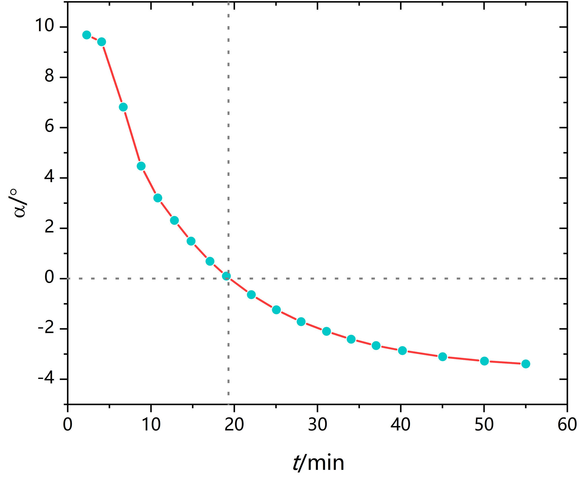
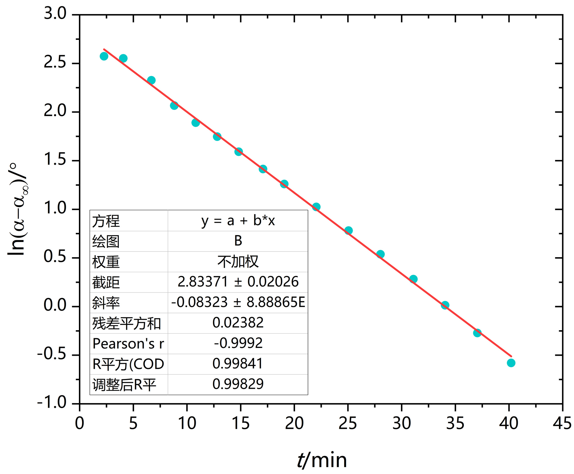
根据P52 2. 作α-t图和4. 作ln[(α-α∞)/°]-t作图，因此，实验报告是两个图，不要遗漏！
4.作ln[(α-α∞)/°]-t作图时，用y = kx + b线性方程拟合。

警告

蔗糖水解反应是一级反应，速率常数k的单位是min-1。
半衰期是min。
实验报告上这两个单位不要遗漏！

Origin作图

虚线不是必须，只是方便显示在19~20 min，旋光度由正变负。

Python作图

2. 作α-t图代码：

 1
 2
 3
 4
 5
 6
 7
 8
 9
10
11
12
13
14
15
16
17
18
19
20
21
22
23
24
25
26
27
28
29
30
31
32
33
34
35
36
37
38
39
40
41
42
43


import matplotlib.pyplot as plt

# 数据
data = """
2.28    9.684
4.07    9.411
6.68    6.816
8.82    4.47
10.82   3.202
12.82   2.31
14.82   1.486
17.08   0.686
19.06   0.1
22.05   -0.638
25.06   -1.24
28.03   -1.713
31.1    -2.099
34.05   -2.411
37.05   -2.662
40.2    -2.864
45.03   -3.107
50.05   -3.278
55.02   -3.391
"""

# 解析数据
lines = data.strip().split("\n")
x, y = zip(*[map(float, line.split()) for line in lines])

# 绘图
plt.plot(x, y, color='tab:red', label='Line through Data Points')
plt.scatter(x, y, color='tab:blue', label='Data Points')
plt.xlabel('t/min')
plt.ylabel(r'$\alpha$' + '/°')
plt.legend()
plt.grid(True)

# 保存为300dpi的图像
plt.tight_layout()
plt.savefig("C:\\Users\\lenovo\\Desktop\\pic1.jpg", dpi=300)

# 显示图形
plt.show()

2. 作α-t图作图：

4. 作ln[(α-α∞)/°]-t代码：

 1
 2
 3
 4
 5
 6
 7
 8
 9
10
11
12
13
14
15
16
17
18
19
20
21
22
23
24
25
26
27
28
29
30
31
32
33
34
35
36
37
38
39
40
41
42
43
44
45


import numpy as np
import matplotlib.pyplot as plt

# 数据
data = """
2.28    2.57322
4.07    2.55218
6.68    2.3263
8.82    2.0661
10.82   1.891
12.82   1.74641
14.82   1.59127
17.08   1.41342
19.06   1.2596
22.05   1.02461
25.06   0.78116
28.03   0.53708
31.1    0.28141
34.05   0.01292
37.05   -0.27181
40.2    -0.57982
"""

# 解析数据
lines = data.strip().split("\n")
x, y = zip(*[map(float, line.split()) for line in lines])

# 使用numpy进行线性拟合
coefs = np.polyfit(x, y, 1)
fit_func = np.poly1d(coefs)

# 绘图
plt.scatter(x, y, color='tab:blue', label='Data Points')
plt.plot(x, fit_func(x), color='tab:red', label=f'Fit: y = {coefs[0]:.4f}x + {coefs[1]:.4f}')
plt.xlabel('t/min')
plt.ylabel(r'ln($\alpha$-$\alpha_{\infty}$)/°')
plt.legend()
plt.grid(True)

# 保存为300dpi的图像
plt.tight_layout()
plt.savefig("C:\\Users\\lenovo\\Desktop\\pic2.jpg", dpi=300)

# 显示图形
plt.show()

4. 作ln[(α-α∞)/°]-t作图：

Matlab作图

2. 作α-t图代码：

 1
 2
 3
 4
 5
 6
 7
 8
 9
10
11
12
13
14
15
16
17
18
19
20
21
22
23
24
25
26
27
28
29
30
31
32
33
34
35
36
37
38
39


% 数据
data = [
    2.28, 9.684;
    4.07, 9.411;
    6.68, 6.816;
    8.82, 4.47;
    10.82, 3.202;
    12.82, 2.31;
    14.82, 1.486;
    17.08, 0.686;
    19.06, 0.1;
    22.05, -0.638;
    25.06, -1.24;
    28.03, -1.713;
    31.1, -2.099;
    34.05, -2.411;
    37.05, -2.662;
    40.2, -2.864;
    45.03, -3.107;
    50.05, -3.278;
    55.02, -3.391;
];

% 提取x和y
x = data(:, 1);
y = data(:, 2);

% 绘图
figure;
plot(x, y, '-r', 'DisplayName', 'Line through Data Points');
hold on; % 保持当前图形
scatter(x, y, 'blue', 'DisplayName', 'Data Points');
xlabel('t/min');
ylabel('\alpha/°');
legend;
grid on;

% 保存为300dpi的图像
print('C:\Users\lenovo\Desktop\pic1.jpg','-djpeg','-r300');

2. 作α-t图作图：

4. 作ln[(α-α∞)/°]-t代码：

 1
 2
 3
 4
 5
 6
 7
 8
 9
10
11
12
13
14
15
16
17
18
19
20
21
22
23
24
25
26
27
28
29
30
31
32
33
34
35
36
37
38
39
40


% 数据
data = [
    2.28, 2.57322;
    4.07, 2.55218;
    6.68, 2.3263;
    8.82, 2.0661;
    10.82, 1.891;
    12.82, 1.74641;
    14.82, 1.59127;
    17.08, 1.41342;
    19.06, 1.2596;
    22.05, 1.02461;
    25.06, 0.78116;
    28.03, 0.53708;
    31.1, 0.28141;
    34.05, 0.01292;
    37.05, -0.27181;
    40.2, -0.57982;
];

% 提取x和y
x = data(:, 1);
y = data(:, 2);

% 使用MATLAB的polyfit进行线性拟合
coefs = polyfit(x, y, 1);
fit_values = polyval(coefs, x);

% 绘图
figure;
scatter(x, y, 'blue', 'DisplayName', 'Data Points');
hold on;
plot(x, fit_values, 'red', 'DisplayName', sprintf('Fit: y = %.4fx + %.4f', coefs(1), coefs(2)));
xlabel('t/min');
ylabel('ln(\alpha-\alpha_{\infty})/°');
legend;
grid on;

% 保存为300dpi的图像
print('C:\Users\lenovo\Desktop\pic2.jpg','-djpeg','-r300');

4. 作ln[(α-α∞)/°]-t作图：

目录

《物理化学实验》-生态环境系

电导法测定弱电解质的电离平衡常数

实验思路

数据处理

Origin作图

Python作图

Matlab作图

Mathematica作图

Julia作图

蔗糖转化反应速率常数的测定

实验思路

数据处理

Origin作图

Python作图

Matlab作图